PSF Estimation Modeling and Non-Blind Deconvolution of Photos with Spatially-Variant Motion Blur Through Inertial Sensor Data
The source code for this project is available to download on GitHub. Additionally, the thesis document that this project was built for can be accessed from here.
Introduction
The image motion deblurring project I did during my time at the University of Pennsylvania (which I discussed here). has the capability to remove spatially-variant motion blur from images. However, they are trained on motion data that are simple; i.e., linear. In other words, the blur kernels for the images are straight lines. Additionally, they assume a constant acceleration in the rotational and translational movements of the camera.
It is theoretically possible to train a CNN to remove motion blurs with kernels shaped like, say, a tangled thread. But two problems arise when we try to do so. First, the number of parameters needed (the number of base channels, that is) would need to be much larger than what I had in that motion deblurring project. Secondly, an entirely new way would be needed to encode non-linear motion data such that they can be concatenated to the image tensor. The second one proves to be more difficult by far.
Approaching the time for my undergraduate thesis proposal, I revisited the idea of motion deblurring. I went back to the original reason I started my exploration into the topic: reversing motion blur that naturally occurs when taking photos with consumer-grade cameras. In the image deblurring project I did at Penn, I felt that I wasn’t able to retrieve enough fine details from the blurry image for it to be usable for everyday consumer-grade use; I saw it more as a proof-of-concept.
Having perused the deconvolution literature for weeks during my time in the US, I saw another avenue in approaching image deblurring: through the use of non-blind deconvolution algorithms. However, they tend to be far more sensitive to noise compared to AI-based methods: having the value of the estimated kernel off by a slight amount can derail the deblurring result.
So I needed a robust way to model what the kernel of a blurred image would look like given motion data with non-constant acceleration.
I ended up taking on this project as the topic for my undergraduate thesis, which can be accessed through here. Its purpose is to create an image deblurring solution that more reliably recover details, through the use of highly accurate kernel estimation and a non-blind deconvolution algorithm.
Background Knowledge
Most of the theoretical basis this project is built from have been discussed in this page. So, the only part left to be discussed here is the concept of non-blind deconvolution algorithms.
Through reading research and experimenting myself I learned that “Fourier deconvolution” (and most of its derivatives, like the Wiener filter) doesn’t apply too well for real-world image motion deblurring. This is mostly because real-world blur kernels can be non-linear and complex in shape—which means simplifying them as mere lines can destabilize the deconvolution process.
Unlike with an AI-based approach, the tolerance for kernel estimation accuracy is much lower. This project focuses on tackling that issue. Which is why, a more noise-tolerant deconvolution algorithm is needed.
The specific algorithm used is the Wiener-Hunt deconvolution algorithm. It is one of the many evolutions of “Fourier deconvolution” (you can read about this here on p. 12–15). It uses a Bayesian MCMC (Markov Chain Monte Carlo) approach with Gibbs sampling. At its core, it works by sampling from the posterior distribution of possible images and returns the posterior mean as the deconvolved image.
Problem Statement
This project aims to create an image deblurring pipeline that is focused on getting kernel estimation to be as accurate as possible. The structure of the pipeline is shown in the figure below.

This project’s original contribution, albeit relatively small one, to the image deconvolution literature is also shown here: an algorithm that converts motion data into Point Spread Functions (PSF)—which is what kernels are often referred to in the context of image deblurring. From this section forwards, I will also start to refer to kernels as PSFs.
For this project, I also made a simple pixelization algorithm which converts a point in the Cartesian plane to pixels. Unlike other vector-to-pixel algorithms, this one is designed from the ground up to work in tandem with the motion-to-PSF algorithm that is introduced here.
Methodology
Python is used as the project’s main language, with MATLAB to capture the motion sensor data of an iPhone 13. NumPy, SciPy, SciKit Image, and OpenCV are the main libraries used here.
The capturing of motion data and the creation of the homography matrices are mostly the same as the one mentioned here. With that project, however, the only motion data captured is at the moment when the camera shutter opens and at the moment when it closes.
Projective (or homography) transformation is then used to calculate the change that each point in the image plane experiences after the rotation and/or translation.
With this project, the transformations are computed for intermediate points between the start and the end as well. Because of this, the resulting PSFs doesn’t have to be reduced to just straight lines—they can be shaped like tangled threads if they need to be. The figure below shows what a PSF with a complex shape and non-constant acceleration can look like:
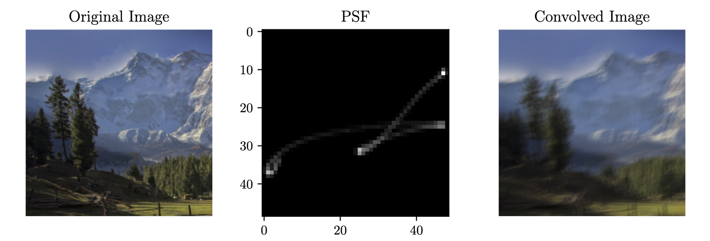
This is a departure from the simple idea of a PSF (blur kernel) introduced here.
The multi-homographies employed here is only one part of the story in getting a PSF model that accurately reflects its real-world counterpart. There are two main things to be noted in the PSF image on the top figure: (1) the difference in luminosity in different parts of the non-linear line, and (2) the fact that the luminosity of overlapping parts are consistent with the number of overlaps.
In the real world, the movements that cause motion blur is almost never of a constant acceleration—they slow down and speed up. It is natural that parts of the PSF that are traced by the slower movements will appear brighter. And, when the PSF line crosses the same place more than once, their brightness should be additive of each other.
The motion-to-PSF algorithm (referred to as Algorithm 1 in my thesis) uses an intuitive way to have these two properties encoded into the final PSF.

In it, a PSF goes through an intermediate Cartesian form before being pixelated into its matrix form. They can be mathematically formalized as the vector-valued function
where and are the component functions showing the - and -based displacement of the point of interest during the homography transformation.
Each points in the function is then converted into pixels using the pixelization algorithm (referred to as Algorithm 2 in my thesis). Here’s a gist of how it works. A grid of size is first defined on the Cartesian plane. By default, .
Every point in the vector-valued function projects what I call a psuedo-pixel, which is marked in red in the bottom figure.
The area of that pseudo-pixel that encroaches on a particular grid box can be calculated through the following formula:
That resulting area, , is used to determine the brightness of the pixel represented by the grid box of interest.
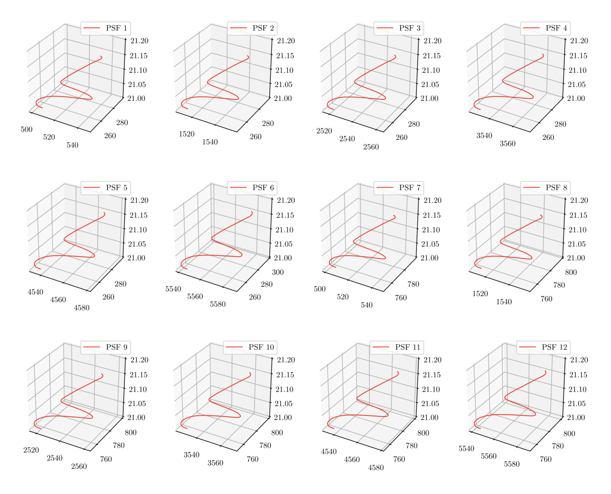
This calculation is repeated for every points defined in the domain of . The result is shown in the figure to the bottom right. (Here, the image is divided into subdivisions, each with their own PSF).
The fact is, that for every , will fall within some grid boxes more often than others. This naturally allows pixels to have higher luminosity than others. The nature of the pixelization algorithm also gives to the resulting PSF models an anti-aliasing effect—which is desirable.
Results and Discussions
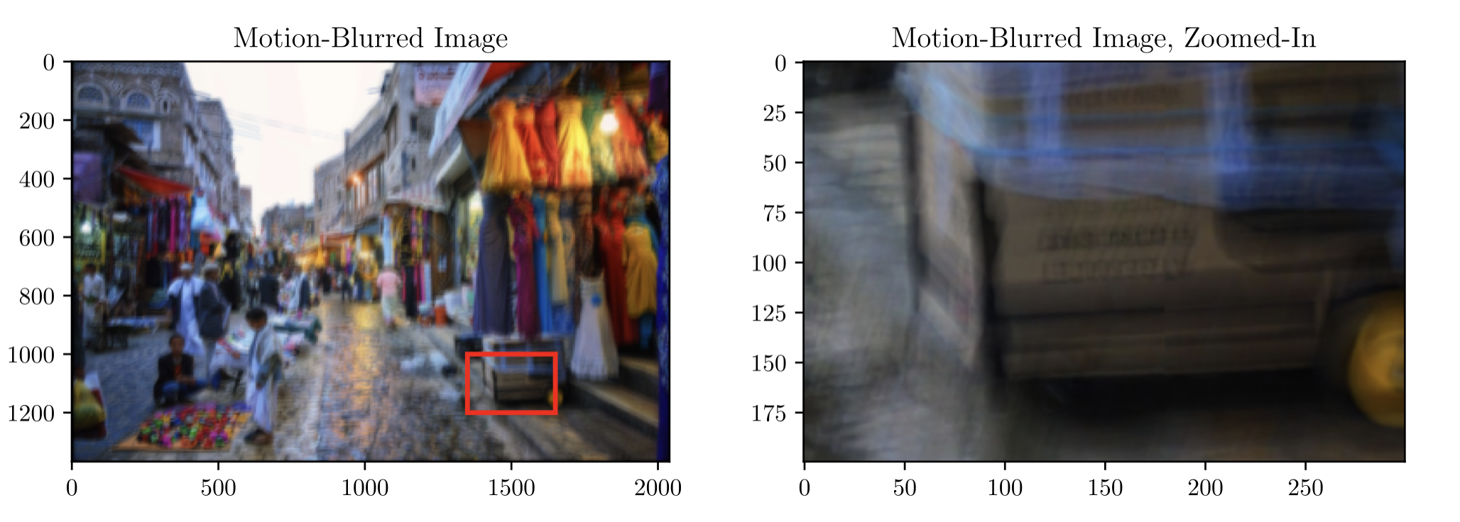
The images below shows the result of the deblurring using this pipeline.
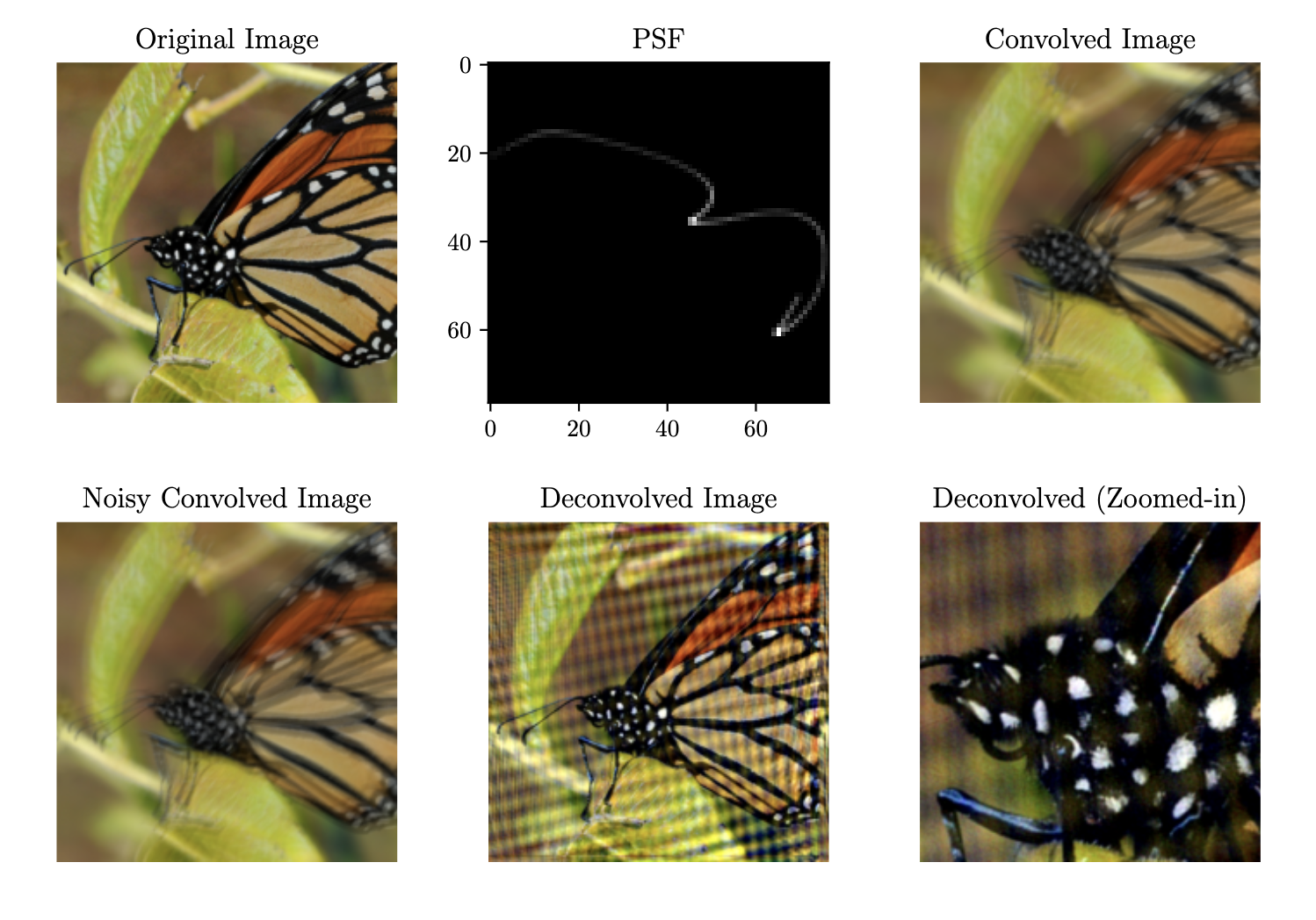
It manages to retrieve fine details from images with minimal loss. The average Spatial Similarity (SSIM) between deconvolved images and ground truth images are 0.881. The PSF models were also found to have a very high similarity to their real-world counterparts, with an SSIM score of 0.901. (I discussed this here in my thesis on pp. 50–51).
However, the deblurring results does visibly exhibit some artifact, as shown in the figure below. Even with that, it still showcases the amount of detail that the pipeline was able to recover. The testing performed for this project uses motion data that was generated through intentionally excessive movements. In the real-world, most motion blur PSFs aren’t this complex in shape.
Below is a the deblurring result from the pipeline when the motion data is more reflective of real-world situations:
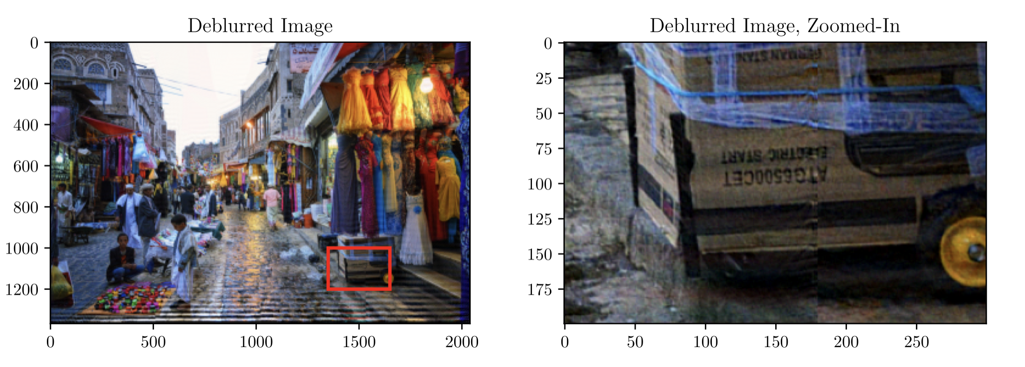
The deblurring result managed to recover details to the extent where ineligible texts in the blurred image becomes readable.
Lessons and Reflections
In completing my thesis, I spent approximately a semester working on this pipeline. When I started, I thought that I already had most of the prerequisite knowledge that I would’ve needed to see this project through. It turns out that I didn’t.
It became clear to me that for a research of this scale, a lot more studying is needed. I spent a considerable amount of time in figuring out the best way to convert the motion sensor data so that it produces the most accurate possible PSFs. I ended using a univariate spline interpolation to turn the data into its continuous form. This is because the motion sensor records data through discrete sampling according to a set frequency. The photographs, though, may be taken at a point in time that happens to not be sampled by the motion sensor. Which is why I ended up deeming the interpolation necessary.
Pursuing this project also pushed me to do more independent learning than I had ever done before (seeing that this is my undergraduate thesis). I was not able to find any literature that detailed the construction of a PSF (or kernel) that realistically describes motion blur. This is why I decided to construct my own algorithm to do so. The pre-defined functions included in NumPy was a huge help in manipulating high-dimensional tensors. (Because of this experience, NumPy array shapes, indexing, and slicing, is now second nature to me.) The process of developing this algorithm wasn’t without its failures, though. For one, I experienced a lot of silent errors that made it really hard for me to debug what’s going on. Needless to say, most of those problems stems from wrong indexing logic—array dimensions get a lot harder to to keep track of once you go beyond three.
I also couldn’t find any vector-to-pixels algorithm that has the properties I described earlier, which is the ability to capture the relationship between movement acceleration differences (and movement overlap) and pixel brightness. Which is why I decided to, again, construct another one of my own. It initially started as just the pixelization algorithm—I actually planned to handle those two properties through another component. Seeing things fall into place with that pixelization algorithm (those two properties turns out to be a naturally-occurring side effect, so I didn’t need to handle them separately) was one of the most satisfying moments in working on this project.
In retrospect, there are a number of things that I could’ve done to make the deblurring result even better. For one, there is the fact that the artifacts sits more on top of the result image rather then blending with its fine details. This is a low hanging fruit that should be solvable through a CNN. The model would only needs to remove the ringing and leave the underlying details untouched. It wouldn’t have to reconstruct any details from minimal information.