Image Motion Blur Removal using Inertial Sensor Data and CNN

The source code for this project is available to download on GitHub.

Introduction

Back when I was in elementary school, I got my first DSLR camera. When taking a photo with it in low-light, my hands had to be really stable, or else I’d get motion blur in my photos.

That was a camera from way back in 2015. Technology nowadays have undoubtedly improved. (An ISO of 25,000 can still get you a usable picture these days.) But, smaller sensors—like the ones we have in embedded systems—don’t have the luxury of cranking up their ISO to compensate for the lack of light.

Because of my early experience with photography, the idea of motion blur removal using motion data had always been sitting in my head. But, it’s only when I went on an exchange to the University of Pennsylvania and got the necessary knowledge that I started actually pursuing it.

This was a project that I did for the final project assignment on the course CIS 5810: Computer Vision & Computational Photography. It’s aimed at removing motion blur from photos, using inertial sensor data as an auxiliary information to guide the restoration process.

Background Knowledge

Many blur effects that are applicable to images can be mathematically modeled through discrete convolution, which is denoted by the $\otimes$ operator. In the eyes of math, a blurred image $B$ is

where $I$ is the latent image, $k$ is the kernel, and $\epsilon$ is an additive noise term applied to every pixel. (The mathematical breakdown of convolution is discussed in my thesis here on pp. 10–12.)

In the context of image processing, the kernel ($k$) is a 2D matrix of an arbitrary size that can be convolved with $I$, an image (also a 2D matrix) to create all kinds of effects. Gaussian blurs, for example, is produced through convolution, which is shown in the figure below.

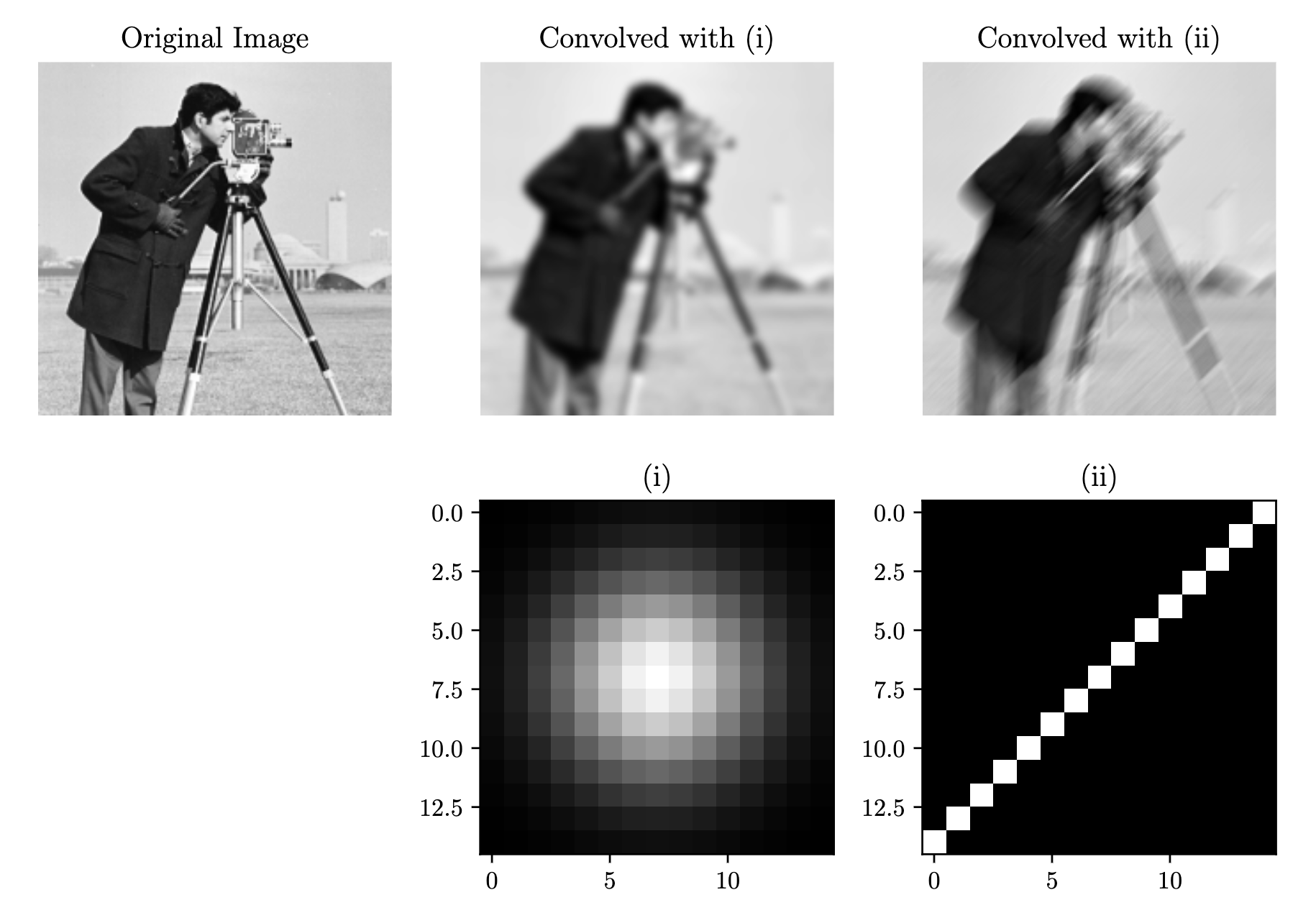
The kernel (i) is called the Gaussian kernel. Motion blurs, on the other hand, are produced by kernels with a more line-like shape, such as (ii). As seen in the resulting image, the motion blur follows a bottom-left-to-top-right pattern of motion blur, which reflects what kernel (ii) looks like.

Intuitively, convolution here can be thought of as taking an image and spreading each pixel throughout that image according to the kernel’s specifications. Which is why the kernel is known by another name: the Point Spread Function (PSF).

Convolution has an inverse—what is convolved can be deconvolved using a process called, well, deconvolution. A non-blind deconvolution is where we attempt to recover the latent image $I$ from $B$ with knowledge of the kernel $k$—or at least an estimate of it. The better the kernel estimate, the better the resulting deconvolved image will be. (You can read more about how deconvolution works mathematically in my thesis here on pp. 12–14.)

This tells us, that for a motion-blurred image $B$, so long as we can estimate the kernel $k$, we should be able to recover the latent image $I$.

In the case of motion blur, we can use an inertial sensor to obtain data about the movement of a camera—which in turns, will help us find the kernel $k$ (otherwise known as a PSF).

There are two kinds of movements we need to think about: rotation and translation. Rotation data is obtained through a gyroscope while translation data is obtained through an accelerometer. The figure on the bottom illustrates the shape of the kernels depending on what kind of movements created them. Notice how there are multiple different kernels for every part of the image. This is called spatial variance.

The lines making up every kernel can be found through projective (or homography) transformation. (You can also read more about this here on pp. 17–18.)

Problem Statement

This project aims to leverage the image restoration ability that CNNs exhibit to remove motion blur from photos. This arrangement is unique because motion sensor data is also included in as a part of the input, rather than just the image.

CNN Architecture

The CNN is of an U-Net architecture. That architecture was chosen for this project because of its encoder-decoder structure. The encoder can capture the motion blur patterns at multiple scales (edges, textures, motion directions). The decoder helps reconstruct the desired sharp details of the latent image.

Another key feature of a U-Net is skip connections. For image restoration processes like this, skip connections are critical to ensure that final model can understand both high-level features of the blurred image (from the bottleneck) and its low-level details like spatial information (from the encoder shared with the decoder).

The figure below shows the exact architecture of the CNN, including the number of channels on each layers and the operations involved to get from one layer to the other.

The input tensor here has 6 channels. This is because of the way the motion sensor data is combined with the image: by concatenation. So, in the input tensor, there are 3 channels dedicated motion data. Those channels are essentially a discrete vector field; where every vector represents a kernel that describes the motion blur for the image in that particular section.

Each of the vectors are broken down into 3 pieces: their magnitudes (also known as norms), $x$ components, and $y$ components. This effectively assigns every pixel in the image, their own kernel in the form of a vector.

Methodology and CNN Training

The CNN was trained using 150,000 blurred images. Each of the blurred images have an associated kernel vector field, and a ground truth image.

Python was the programming language of choice for this project. And PyTorch, NumPy, and OpenCV were the major libraries used.

The base of the dataset is obtained from the ImageNet dataset, which were downscaled and cropped to $256\times 256$.

The dataset for the kernel vector fields are obtained through a WitMotion WT901BLECL motion sensor.

The blurry images were created from the ground truth set, which are convolved with kernels generated from the motion sensor data.

The model was trained with a total of 20 epoch, with a batch size of 16, and a learning rate of $2\times {10}^{-4}$. The number of base channels for this model is 32, which brings the total number of parameters to 7,766,915. Making this a small-to-medium-sized CNN model.

With limited time during the week I was working on this project (the final project was held just before finals week at the University of Pennsylvania), and taking into account the possibility of re-training my model in anticipation of training failures, I decided to cut down the overall training time. I did this by reducing the initially-planned number of epochs from 50 to 20, cutting down on the number of parameters (from over 30,000,000) by lowering the number of base channels, as well as trying for a faster convergence by setting the learning rate up from $1\times {10}^{-4}$ to $1\times {10}^{-4}$.

I tested out the difference between training the model with my laptop’s CPU and an Nvidia GPU provided by Kaggle, and found that using a GPU is over 10 times faster. In total, it took around 20 hours training the model with the hyperparameters specified above. However, before that last training session, I had 2 failed attempts. Each of those attempts took around 18 to 20 hours.

In the first one, I did not scale the norm of the kernel vector fields to be between 0 and 1. Because of that, some of the values were comically large or spills into the negative range.

On the second one, I used only Mean Squared Error (MSE) as the loss function, as it relatively fast to compute. However, the result was not satisfactory because with MSE, sharp edges and fine details gets lost because larger errors are heavily-penalized. So, in my third attempt, I took this into account and made a new loss function that is a combination of L1 and MSE. L1 doesn’t over-penalize like MSE does, leading to preserved textures.

Results and Discussions

The deblurring results of the model can be seen in the figure below.

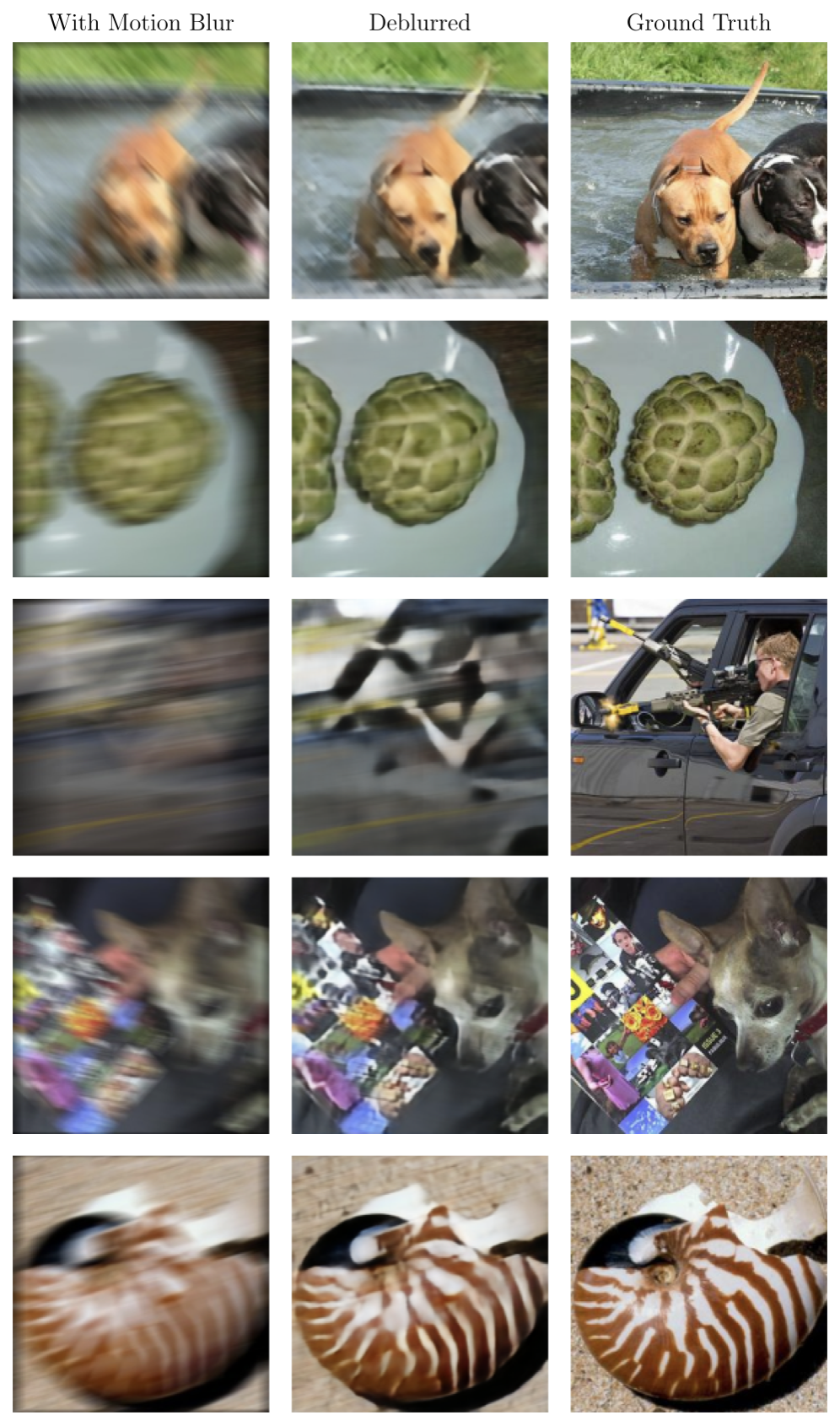
Ten random images were taken from the validation set and was fed into the model. The results shows to have an average Peak Signal-to-Noise Ratio (PSNR) of around 24 dB, which indicates a good deblurring. Out of the 20 epochs, the last one had the best validation loss of 0.0592, with a training loss of 0.0590. The similar values between the training and validation losses indicates that this model generalizes well for images it’s never seen before.

Visually, model is shown to be capable of restoring structure and most textures from blurry images that has almost no fine details visible initially.

The third image shows the amount of textures that can be regained through using the model.

And, with larger and more obstructive motion blurs—as shown in the third image, the model shows that it can regain some structure even if the blurry input image looks like utter nonsense to the human eye.

I acknowledge that the model does not restore 100% of the details from the latent image. That is because this restoration process relies quite heavily on stochastic methods (as all other AI-based solutions do). Even so, it has a number real-world applications. For example, photos exhibiting motion blur can be processed through this model such that it will be repaired to have enough details for use in things like training image classification models.

There is also one important property of this model that adds to its applications: the fact that it doesn’t hallucinate details like some other existing image restoration models. This means, it will never add textures and fine details that weren’t ever there in the first place. This can be extremely useful for the field of forensics, especially in crime scene photo or video analysis.

Lessons and Reflection

Looking back, taking on this project was risky. The CIS 5810 assignment that this CNN model was built for required us to take on something that can be done within approximately two months (including research, planning, and even the search for a suitable dataset). My professor at the time, Jianbo Shi, actually voiced concern in me taking on something this complex alone.

At the time, I haven’t decided yet that the motion deblurring pipeline would involve a CNN. In fact, I wanted to use a method that is purely mathematical; however, I realized that, with my class schedule, two months was not enough time to come up with such deblurring pipeline. During the stage where we were told to decide on what project to pursue, I couldn’t find any paper about motion deblurring that didn’t require any AI-based solution and still offers robust results in the real world. So, at that point, I decided that, employing what I’ve learned in my class there, especially about convolution and CNNs, was the best path forward for this niche topic. (This was also my first time learning about and using a CNN.)

From working on this project, I managed to learn things about image processing that I wouldn’t have otherwise if I had not pursue it. CIS 5810 was a graduate level course (for master’s degree students and PhD candidates), so naturally, even as an undergraduate, I was expected to produce something that is research-grade. To that end, I pushed myself to read a lot of papers that are very much math-heavy.

The most satisfying thing about independent learning from resources like papers, is the eureka moments I’ve had when something clicks—when I managed to figure out unwritten assumptions underlying theories and explanations written there. The weeks that I spent at working on this project is some of the most tiring in my academic life. However, it felt so rewarding that if asked to go through this again, I would do so in a heartbeat.

Although, there are some things that I think I can improve from this model. The first one is a better loss function. The L1-MSE combination I used had an importance ratio of 10 to 1. That is, L1 is considered much more important since it prioritizes sharpness; while MSE acts more like a regularizer. Even with that, they don’t perceive similarities like humans do. So, using loss functions that utilize Structural Similarity (SSIM) or perceptual methods may result in a better penalization—ergo better deblurring.